The transformer paradigm demystified
Notes
- Here is a link to an interesting video to understand the transformer theory: video
Introduction
The transformer paradigm has been first successfully applied in Natural Language Processing (NLP) and is currently highly investigated for image processing.
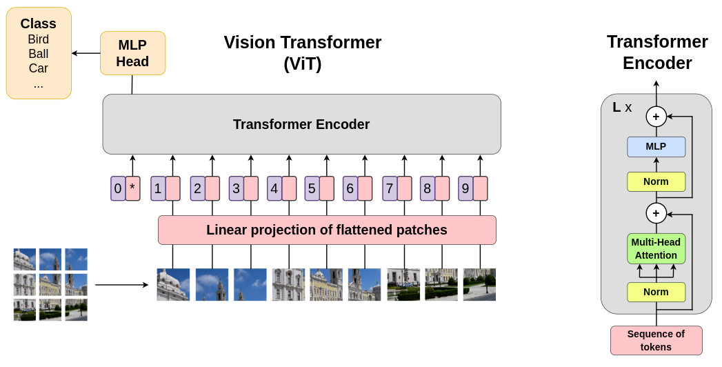
The basic concept of transformers lies in the generation of self attention maps to guide the decision making process of the underlying architecture. To illustrate the underlying mechanism, we will open the black box of the famous Vision Transformer (ViT) method. The overall architecture is given below:
Tokenization process
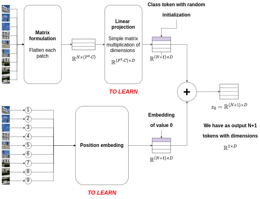
The first step is to convert the input data into a sequence of tokens, i.e. a sequence of vectors of dimensions \(\mathbb{R}^{1 \times (P^2 C)}\), with \(P^2 C\) being the length of each flattened patch. This step is called the tokenization process and involves a simple linear projection (i.e. a multiplication with a matrix of dimensions \(\mathbb{R}^{(P^2 C) \times D}\)) and a position embedding step which encodes spatial information. The same linear projection and position embedding operation are shared to encode each patch. This process is modeled as follows:
\[z_0 = [x_{class}; \, x^1_p\mathbf{E}; \, x^2_p\mathbf{E}; \, \cdots; \, x^N_p\mathbf{E}] + \mathbf{E}_{pos}\]with
\(\mathbf{E}\) being the linear projection matrix of size \(\mathbf{E} \in \mathbb{R}^{(P^2 C) \times D}\)
\(\mathbf{E}_{pos}\) being the output of the position embedding operation with dimensions \(\mathbf{E}_{pos} \in \mathbb{R}^{(N+1) \times D}\)
The figure below illustrates the tokenization process used in ViT.
Transformer encoder
The figure below presents an overview of the encoding layer of a transformer. It is composed of two main steps.
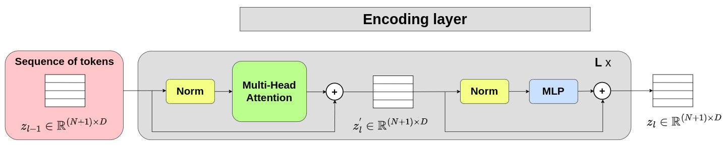
The goal of the first step is to compute attention maps between tokens. The output corresponds to \(z^{'}_l\) which is modeled as follows:
\[z^{'}_l = \text{MHA}(\text{LN}(z_{l-1})) + z_{l-1} \quad \quad \quad \quad l=1 \cdots L\]The goal of the second step is to introduce non-linearities to compute more relevant sequence of tokens. The output corresponds to \(z_l\) which is modeled as follows:
\[z_l = \text{MLP}(\text{LN}(z^{'}_{l})) + z^{'}_{l} \quad \quad \quad \quad l=1 \cdots L\]
Norm step
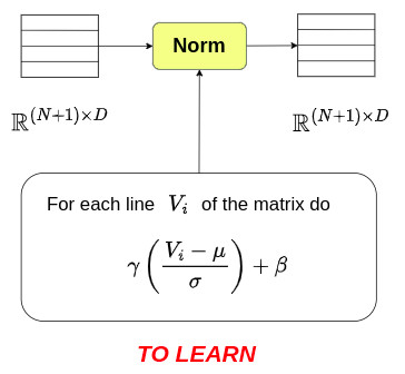
Normalization was inserted into the encoding layer to control the dynamics of the token values before each of the two key steps. The corresponding diagram is given below:
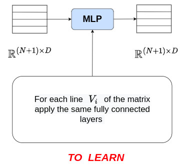
MLP step
The diagram of the \(\text{MLP}\) procedure is given below:
Multi-Head Attention block
The Multi-Head Attention (MHA) block is the key element of the encoding layer. It is based on the “QKV” paradigm, but what does “QKV” mean ? Before answering this question, let’s zoom in on the MHA block and get an overview of its structure.
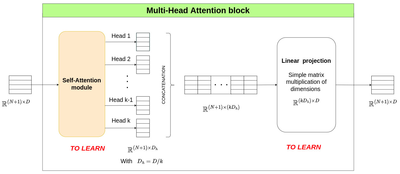
From this figure, we can see that the key element is the Self-Attention module which outputs \(k\) head matrices of size \(\mathbb{R}^{(N+1) \times D_h}\), where \(D_h\) is usually computed as \(D_h=D/k\). These head matrices contain useful information computed from attention mechanisms. The second part of the MHA block uses a linear projection to optimally merge the different heads and to output a new sequence of tokens of the same size as the input matrix, i.e. \(\mathbb{R}^{(N+1) \times D}\). This operation is modeled as:
\[\text{MHA}(z) = \left[ \text{SA}_1(z), \, \text{SA}_2(z), \cdots, \, \text{SA}_k(z) \right] \cdot \mathbf{U}_{msa} \quad \quad \quad \quad \mathbf{U}_{msa} \in \mathbb{R}^{(k D_h) \times D}\]where \(\text{SA}_i(z)\) represents the output of Head \(i\) (\(\text{SA}\) stands for Self Attention). Now it is time to investigate the Self-Attention module !
Self-Attention module
The Self-Attention module is the core element of the MHA block. The figure below provides an overview of such a module.
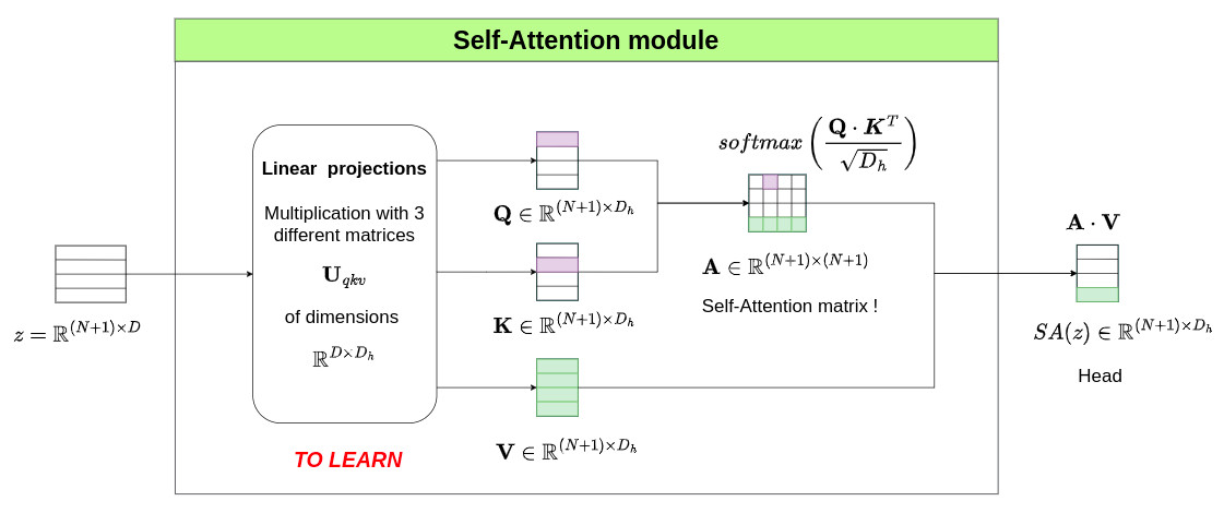
It involves the generation of 3 matrices \(\mathbf{Q}\), \(\mathbf{K}\), \(\mathbf{V}\) of size \(\mathbb{R}^{(N+1) \times D_h}\) computed from three different linear projection matrices \(\mathbf{U}_{qkv} \in \mathbb{R}^{D \times D_h}\). This step is modeled as follows:
\[[\mathbf{Q}, \mathbf{K}, \mathbf{V}] = z \mathbf{U}_{qkv} \quad \quad \quad \quad \mathbf{U}_{qkv} \in \mathbb{R}^{D \times D_h}\]
\(\mathbf{Q}\) and \(\mathbf{K}\) are used to create a self-attention matrix \(\mathbf{A} \in \mathbb{R}^{(N+1) \times (N+1)}\). Since this matrix is computed from scalar products, it expresses the proximity between token \(i\) and all token \(j\). The Softmax operation is applied to each row of \(\mathbf{A}\) individually to ensure that the sum of the elements of each row is equal to \(1\). The corresponding operation is:
\[\mathbf{A} = softmax\left( \frac{\mathbf{Q} \cdot \mathbf{K}^T}{\sqrt{D_h}} \right)\]
Finally, this self-attention matrix \(\mathbf{A}\) is used to compute the final Head matrix \(\text{SA}(z) \in \mathbb{R}^{(N+1)\times D_h}\) whose rows correspond to a weighted sum of the tokens obtained in the \(\mathbf{V}\) matrix. This is done by using the following simple multiplication operation:
\[\text{SA}(z) = \mathbf{A} \cdot \mathbf{V}\]