Transformer Interpretability Beyond Attention Visualization
Note
This paper is in review for ICLR 2021: https://openreview.net/forum?id=YicbFdNTTy
Highlights
Attention weight distribution has received peculiar interest since Transformers became widespread in state-of-the-arts. Analyzing attention weights can bring useful information about the token or the inputs and how they are correlated with the prediction output.
However, gray zones remain. Raw attention has proven to be sometimes irrelevant regarding predictions. The question is “how to rigorously analyse the links between input tokens, attention weights and prediction output?”. Chefer et al. have come up with new leads on this subject, tackling the preexisting issues:
- SOTA methods using raw attention or rollout attention happen to highlight irrelevant tokens
- There are previous methods that propagate attention relevancy down to the attentions heads, to analyse attention heads relevancy separately, but none of these methods propagates the relevancy through all the layer (down to the inputs)
- Layer-wise relevancy propagation (LRP) is a commonly used method to recursively decompose the prediction of the network down to relevance scores for the single input dimensions. But, because of skip connection and attention operators, handling complex activation maps lead to numerical instability, and some amount of the relevancy is lost.
Therefore, the purpose is to get relevant score to be highlighted. The relevancy is assigned to patches and is propagated through all layers of the network, such that:
- the sum of relevancy is maintained throughout the layers
- the method is also class-based, meaning that it provides class-based separation such that the interpretability visualization is not the same regarding the class that is considered (≠ class-agnostic)
- finally, the authors propose a normalization technique to handle the numerical issues entailed by the skip connection and attention matrix multiplication layers
Method
The idea is to employ LRP-based relevance to compute scores for each attention head in each layer. This method incorporates both the relevancy and gradient information such that the negative contribution of a token is iteratively removed.
The relevance propagation follows Deep Taylor Decomposition principle (DTD):
\[R_j^{(n)}=\mathcal{G}(\mathbf{X},\mathbf{Y}, R_i^{(n)}) = \sum_i\mathbf{X}_j\frac{\partial L_i^{(n)}(\mathbf{X},\mathbf{Y})}{\partial \mathbf{X}_j}\frac{R_i^{(n-1)}}{L_i^{(n)}(\mathbf{X},\mathbf{Y})}\]Where $L_i$ denotes the operation between the input feature map $\mathbf{X}$ and the weights $\mathbf{Y}$ for the layer $n$.
⚠️ Notice that the layers are ranked from the output (layer $1$) to the input (layer $N$).
e.g. $L_i(\mathbf{X},\mathbf{Y}) = \sum_{j’}w_{j’i}^+x_{j’}^+$ (LRP, with $(.)^+$ being the ReLU operator), which gives:
\[R_j^{(n)} = \mathcal{G}(x^+, w^+, R^{(n-1)}) = \sum_i \frac{x_j^+w_{ji}^+}{\sum_{j'}x_{j'}^+w_{j'i}^+}R_i^{(n-1)}\]initialized with the one-hot $R^{(0)}=\mathbb{1}_t$ that indicates the target class $t$.
This equation describes the ration between the evolution of $L_i$ and the evolution of $X_j$ for all $i$-th elements in the layer $(n-1)$, multiply for the relevancy score for all previous layers. This equation satisfies the conservation rule:
\[\sum_j R_j^{(n)} = \sum_i R_i^{(n-1)}\]There are two types of layer in a Transformer-type networks:
- parametric layers: involve the mixing of a feature map with a learned tensor $\mathbf{W}$ (typical example: a linear layer in a feed-forward network)
- non-parametric layers: involve the mixing of two feature map tensors. For instance, in a transformer architecture network we have:
- skip connections
- matrix multiplication (in attention modules)
In a self and cross-attention model setup, two feature map tensors are considered (pairwise) : $u$ and $v$. Therefore, the relevance propagation is binary:
\[R_j^{u^{(n)}}=\mathcal{G}(u,v,R^{(n-1)}), \quad R_k^{v^{(n)}}=\mathcal{G}(v,u,R^{(n-1)})\]which are relevances for $u$ and $v$ respectively, the two feature map tensors that are considered. One can notice that the conservation rule is observed when the considered operand is the addition, i.e. $\mathbf{L}^{(n)}(u,v) = u + v$ and then one has:
\[\sum_j R_j^{u^{(n)}} + \sum_i R_k^{v^{(n)}} = \sum_i R_i^{(n-1)}\]But this rule is not observed in general when applying a matrix multiplication ! This brings an instability issue, due to the matrix multiplication and the numerical issues of skip connections. To avoid the relevance scores of $u$ and $v$ exploding, the authors propose a normalization technique such that $\sum_i R_i^{(n)} = 1$ for each layer $n$. Moreover, their normalization techniques upholds the two following properties:
- The conservation rule
- It bounds the relevance sum of each tensor such that:
where $\bar{R}_j^{u^{(n)}}$ and $\bar{R}_k^{v^{(n)}}$ are respectively the normalized term of the previous defined relevancy of $u$ and $v$.
The model is then a Transformer model:
- consisting of $B$ blocks, each one composed of:
- self-attention
- skip connections
- additional linear
- normalization layer (to prevent relevance exploding)
- input: a sequence of $s$ tokens with a [CLS] token for classification
- output: classification probability vector $y\in\mathbb{R}^C$
- self-attention map for the block $b$ is $A^{(b)}=\mathrm{softmax}\left(\frac{\mathbf{Q}^{(b)}\cdot\mathbf{K}^{(b)^T}}{\sqrt{d_h}}\right)$, row-wise
- The relevance of each attention map is computed for the layer where the softmax operation is applied (the layer $n_b$):
Notice that this methods depends of the target class, which was not the case of the previous methods such as rollout attention.
Finally, the matrix $\mathbf{C}$ is used, where $\mathbf{C} \in \mathbb{R}^{s \times s}$ and $s$ is the sequence length. Only the row associated to the [CLS] token is considered, and only the authors keep the $s-1$ tokens that correspond to the actual inputs.
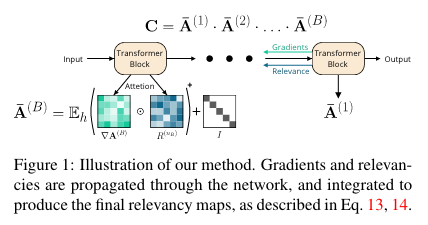
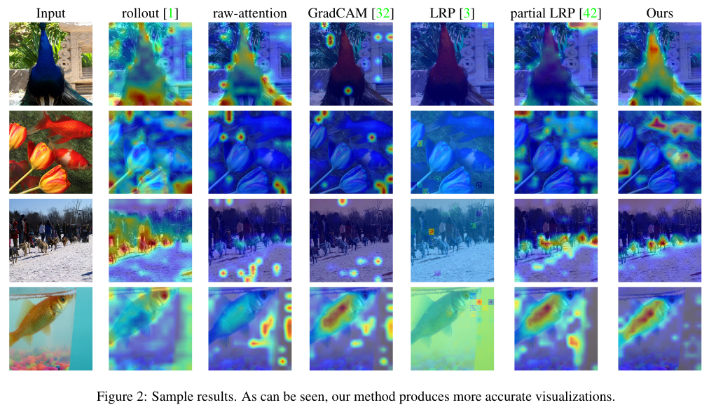
Experiments and results
For images, they used a BERT-like ViT, on non-overlapping patches of $16\times 16$. Two tests are performed:
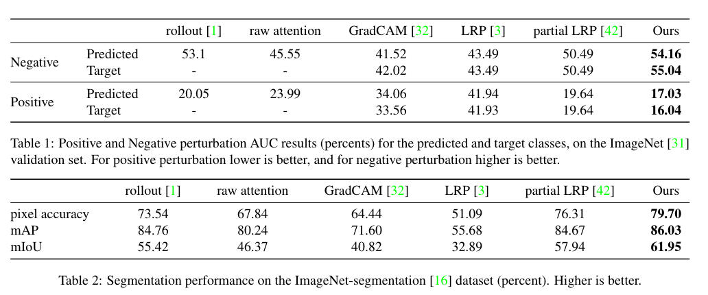
- The positive and perturbations tests (positive perturbation: pixels are masked from the highest relevance to the lowest ; negative perturbations: the other way around)
The evaluation of the model follows this procedure:
- pre-trained network to extract visualizations for the validation set
- gradually mask out the pixels and measure the mean top-1 accuracy of the network
- the AUC is measured while removing pixels to test the drop in performances of the model
- The segmentation tests
Each visualization is considered as a soft-segmentation of the image, and can be compared to the ground truth segmentation (from the ImageNet-Segmentation dataset). Three metrics are used:
- pixel-accuracy: thresholding each visualization by the mean value
- mean Intersection over Union (mIoU)
- mean Average Precision (mAP): uses the soft-segmentation to obtain a score that is threshold-agnostic
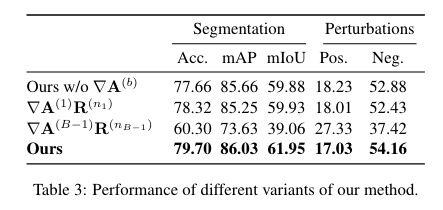
Finally, ablation studies are performed, consisting in removing $\nabla \mathbf{A}^{(b)}$ and replacing it with $\mathbf{A}^{(b)}$ in the relevancy propagation equation, or applying the method in the last block of the model only, or in the first block (respectively closest to the output or closest to the input).